Congratulations on your purchase of an Infix-2!
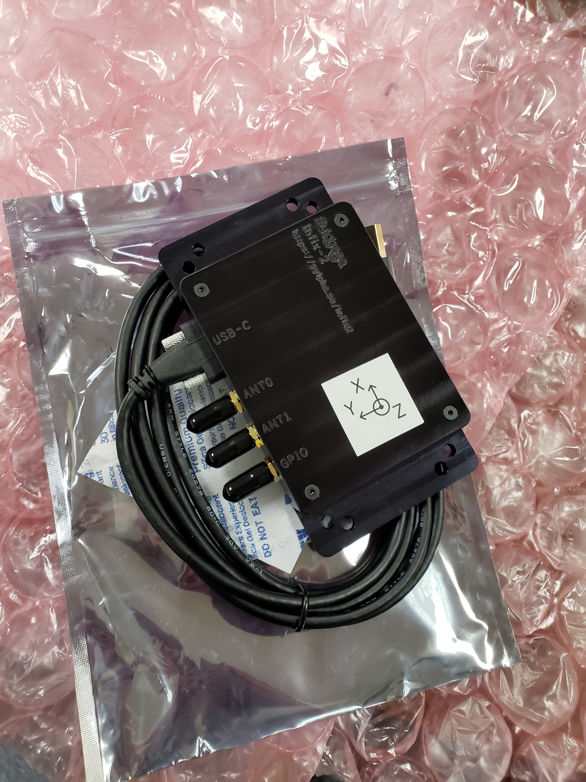 |
| Infix-2 with packaging |
The Infix-2 PCB is mounted in an anodized aluminum case. The case has an axis reference that specifies the coordinate system used by the IMU and magnetometer. The case has the following hole patterns for mounting:
The Infix-2 device has the following labelled ports:
USB-C - USB-C port for connecting to host computer for power and USB 2.0 dataANT0 - SMA primary antenna RF inputANT1 - SMA secondary antenna RF input--use-ant1GPIO - SMA general purpose input/output--output-pps)--use-pps) or 5 MHz reference (--use-pll)All ports are ESD-protected.
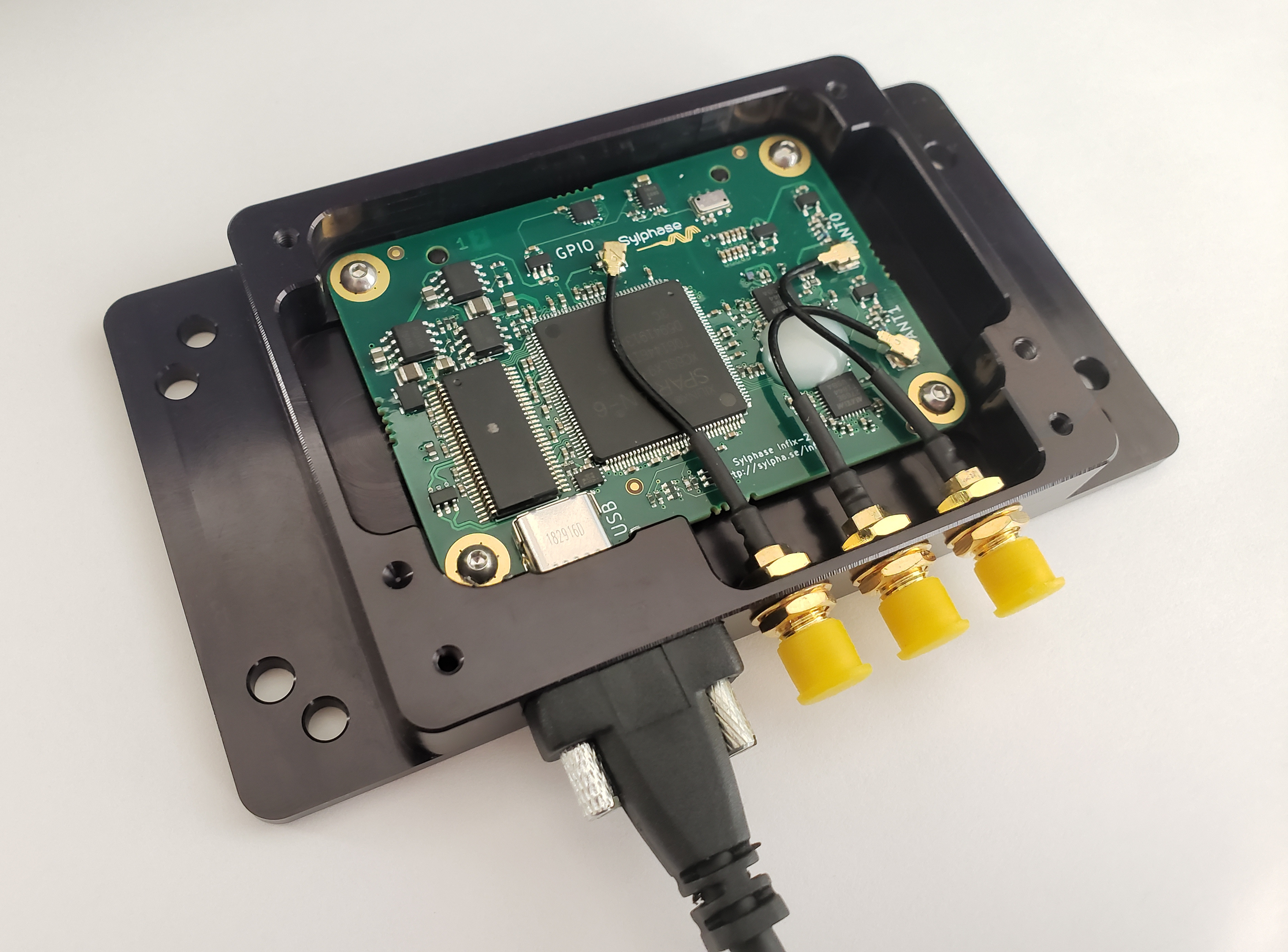 |
| Infix-2 case opened (Note: SMA port ordering has changed since this picture was taken.) |
At this point, you should be able to run sdgps and get tab-completion. Try typing sdgps <TAB><TAB> and you should get a list of SDGPS's global options and nodes that can be used at the start of a pipeline.
Now, let's do a simple test to make sure the hardware is working. Run:
sdgps \
    sylphase-usbgpsimu2-raw \
    ! plot-sensors
After a few seconds, a live plot should pop up that has measurements from all the internal sensors. Try exciting all the sensor axes by rotating the device. The barometer can be tested by moving the device up and down by at least a meter.
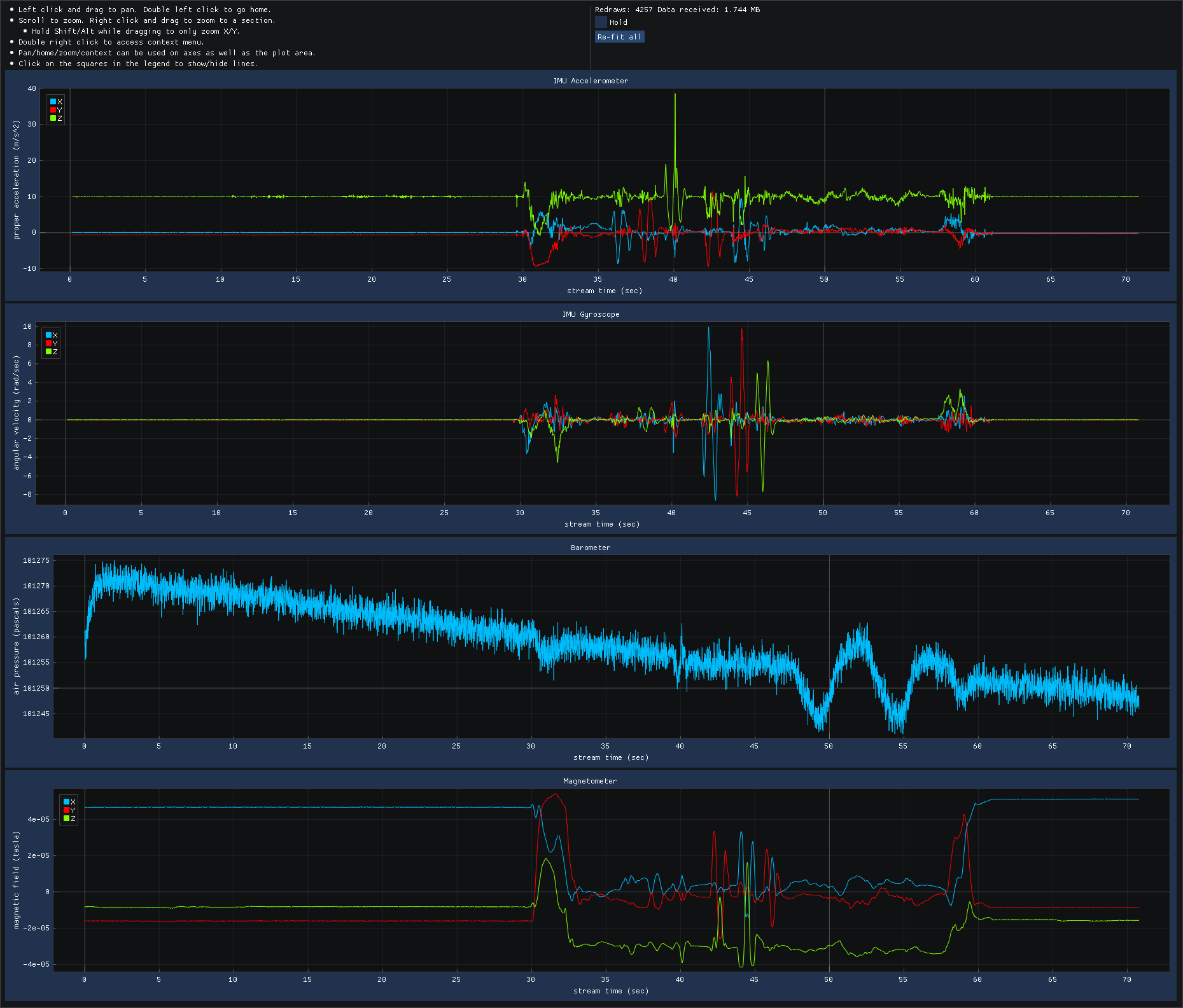 |
| Example output of plot-sensors node |
The console output should look like the following:
Run the following command:
sdgps \
    sylphase-usbgpsimu2-raw \
    ! plot-raw
Now, you should see a power spectral density plot. If you don't have an antenna plugged in or if you're inside and the antenna is near any potential interference source (e.g. a computer), you might see spikes in the PSD plot. However, during normal operating conditions, the plot should look relatively clean, with minimal spurs.
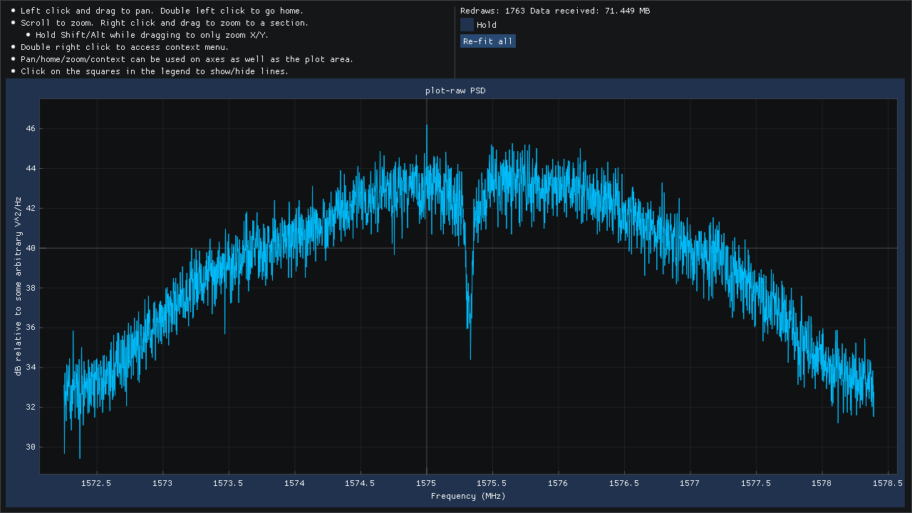 | 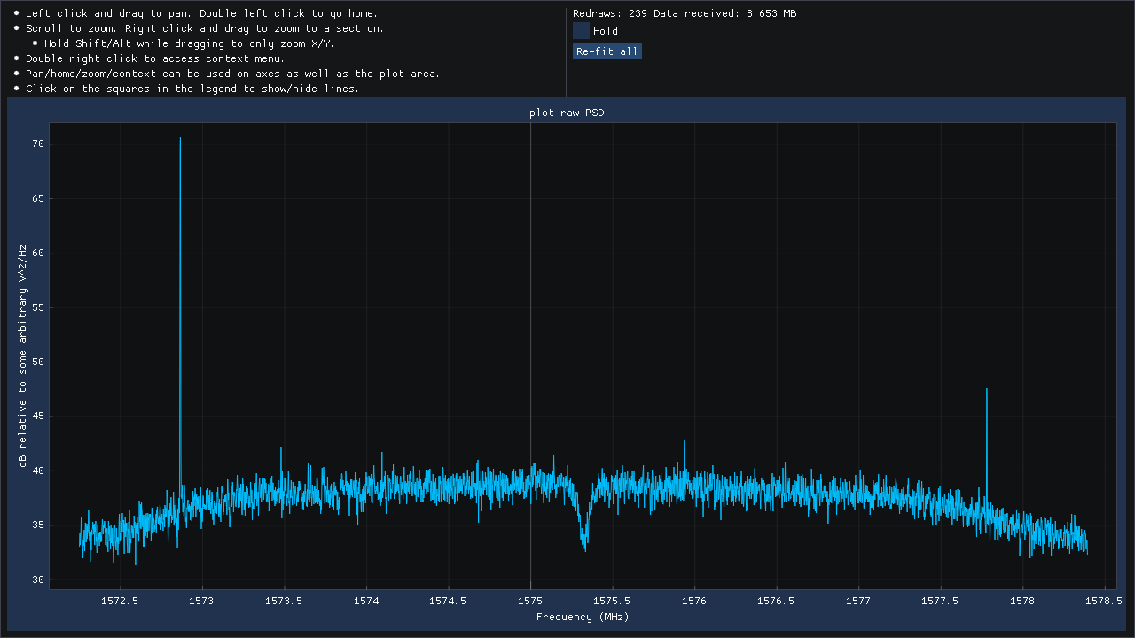 |
| Example output of plot-raw node (with antenna plugged in and viewing sky) | Example output of plot-raw node (with no antenna plugged in) |
Now that the device is known to be operating correctly, let's do an outside data capture. Connect the antenna to ANT0 and run the following command:
sdgps \
    sylphase-usbgpsimu2 --antenna-position '[0,0,0]' \
    ! tracker \
    ! decoder \
    ! write-observables-file capture1.obs \
    ! plot-observables --detrend
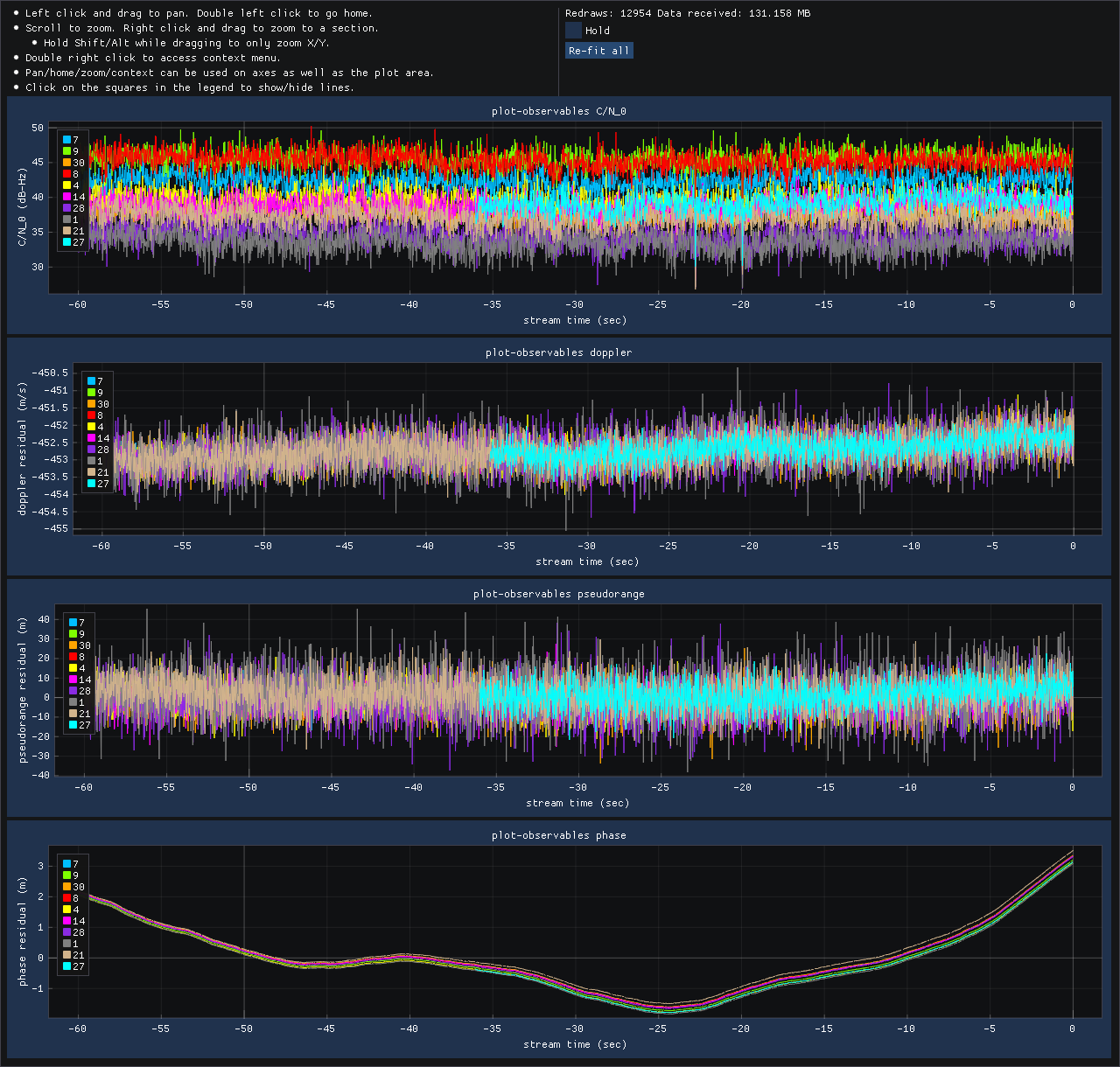 |
| Example output of plot-observables node |
The system should begin acquiring and tracking SVs. The status line displayed at the bottom of the console has the following format:
[ACQ# 1.98] [time: 52.69] [GPS_L1 9/10] [GPS_L1 7/9]
[ACQ# 1.98] - So far, 1.98 full acquisitions have completed.[time: 52.69] - The receiver time is 52.69 seconds.[GPS_L1 9/10] - Out of the 10 SVs being tracked, data bit alignment has completed for 9 of them.[GPS_L1 7/9] - Out of the 9 SVs for which alignment has succeeded, 7 have a valid ephemeris and are generating observables.After about 60 seconds, a line like ...
plot-observables: Computed position-ecef: [-521830.21008324844,-5521417.7063672524,3139403.0775780249]
... will be printed, signifying that the first fix has been obtained. At that point, the observables plot should begin updating.
For the purposes of this tutorial, please record for at least a few minutes without moving or otherwise disturbing the antenna.
If we can assume that the antenna was stationary, we can now use the static-kf2 node to filter the observables into a good solution:
sdgps \
    read-observables-file capture1.obs --rate inf \
    ! static-kf2 --output-rate 10 \
    ! plot-solution --detrend
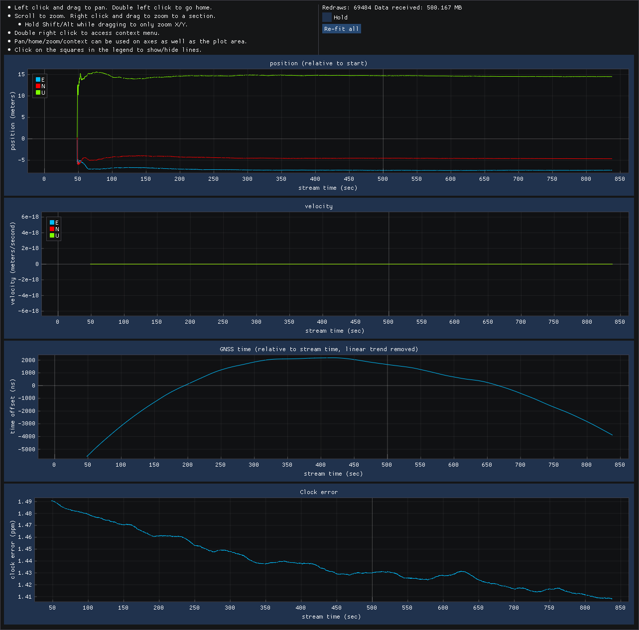 |
| plot-solution plot of static-kf2 's output |
As we can see in the results pictured on the right, position varies at the start, but quickly converges and then stays very constant, as expected of the static position assumption.
If we can't assume that the antenna was stationary and we don't want to use the inertial sensors, then we have to use the simple-pvt-solver node, which does single-point GNSS solutions (no filtering at all).
sdgps \
    read-observables-file capture1.obs --rate inf \
    ! simple-pvt-solver --output-rate 10 \
    ! plot-solution --detrend
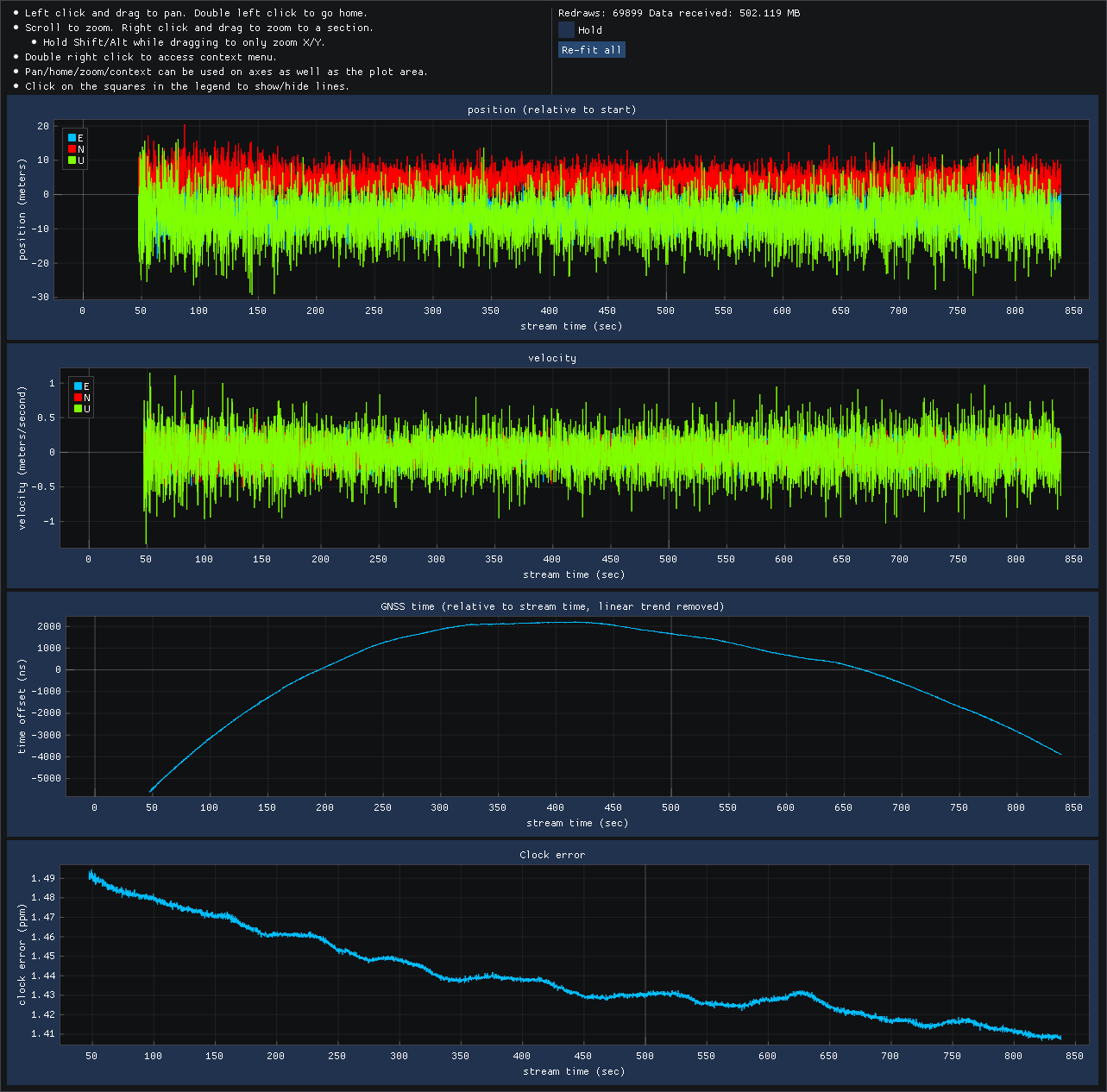 |
| plot-solution plot of simple-pvt-solver 's output |
As we can see in the results pictured on the right, the results match those of static-kf2, except for there being significantly more noise. The vertical "U" component of position is noisiest. It can be hidden in the plot by clicking on its square in the legend.